 A graph illustration
Graph Base SLAM Introduction
Table of Contents
Introduction
Graph based SLAM also known as least square approach. It’s an approach for computing solution for overdeterminined systems by minimizing the sum of squared errors. It has been proposed earlier in the year of 1997. However, it took several years to make this formulation popular due to the relatively high complexity of solving the error minimization problem using standard techniques.
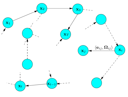
Graph
The graph in the method contains two parts:
- Nodes: nodes in the graph correspond to the poses of the robot at time $t_1, t_2, t_3…,t_k$
- Edges: edges in the graph represent the constraints between poses. The edge usually encodes the sensor measurement that constrains the connected poses.
Observation function
The final goal of SLAM problems is calculating the map and the trajectory of the robot based on the data we get from the sensors.
The observation function is that: at time $k$ the robot at position $x_k$, gets data $z_k$ from the sensor:
\begin{equation}{z_k} = h\left( {{x_k}} \right) \end{equation}
As errors exist in the observation process, our goal is to optimize the error between the actual observations and the observations perceived by the sensors
Graph based SLAM pipeline:
- Constructing the graph(Front end)
- Graph optimization(Back end)
def GBS():
  construct_graph()
  optimize_graph()
  return
Graph Based SLAM Practice
Compile g2o from source and install
clone g2o from github and use CMake to compile and install
git clone https://github.com/RainerKuemmerle/g2o && cd g2o
CMake and make
cmake . && make
make install
sudo make install
Use g2o to fit curves
The function we’re going to fit is:
$$y = e^{3.5x^3+1.6x^2+0.3x+7.8}$$
Pipeline of graph optimization process
- Defining type of the
nodesandedgesin the graph - Contructing the
graph Rotationandoptimizationalgorithm- Apply g2o and get results that are returned from g2o
FindG2O.cmake from where you build your g2o library to the folder where you want to build the following source code
main.cpp
#include <iostream>
#include <g2o/core/base_vertex.h>//顶点类型
#include <g2o/core/base_unary_edge.h>//一元边类型
#include <g2o/core/block_solver.h>//求解器的实现,主要来自choldmod, csparse
#include <g2o/core/optimization_algorithm_levenberg.h>//列文伯格-马夸尔特
#include <g2o/core/optimization_algorithm_gauss_newton.h>//高斯牛顿法
#include <g2o/core/optimization_algorithm_dogleg.h>//Dogleg(狗腿方法)
#include <g2o/solvers/dense/linear_solver_dense.h>
#include <Eigen/Core>//矩阵库
#include <opencv2/core/core.hpp>//opencv2
#include <cmath>//数学库
#include <chrono>//时间库

using namespace std;

//定义曲线模型顶点,这也是我们的目标优化变量
//这个顶点类继承于基础顶点类,基础顶点类是个模板类,模板参数表示优化变量的维度和数据类型
class CurveFittingVertex: public g2o::BaseVertex<4, Eigen::Vector4d>
{
public:
    //因为类中含有Eigen对象,为了防止内存不对齐,加上这句宏定义
    EIGEN_MAKE_ALIGNED_OPERATOR_NEW

    //在基类中这是个=0的虚函数,所以必须重新定义
    //它用于重置顶点,例如全部重置为0
    virtual void setToOriginImpl()
    {
        //这里的_estimate是基类中的变量,直接用了
        _estimate << 0,0,0,0;
    }

    //这也是一个必须要重定义的虚函数
    //它的用途是对顶点进行更新,对应优化中X(k+1)=Xk+Dx
    //需要注意的是虽然这里的更新是个普通的加法,但并不是所有情况都是这样
    //例如相机的位姿,其本身没有加法运算
    //这时就需要我们自己定义"增量如何加到现有估计上"这样的算法了
    //这也就是为什么g2o没有为我们写好的原因
    virtual void oplusImpl( const double* update )
    {
        //注意这里的Vector4d,d是double的意思,f是float的意思
        _estimate += Eigen::Vector4d(update);
    }

    //虚函数  存盘和读盘:留空
    virtual bool read( istream& in ) {}
    virtual bool write( ostream& out ) const {}
};


//误差模型—— 曲线模型的边
//模板参数:观测值维度(输入的参数维度),类型,连接顶点类型(创建的顶点)
class CurveFittingEdge: public g2o::BaseUnaryEdge<1,double,CurveFittingVertex>
{
public:
    EIGEN_MAKE_ALIGNED_OPERATOR_NEW
    double _x;

    //这种写法应该有一种似曾相识的感觉
    //在Ceres里定义代价函数结构体的时候,那里的构造函数也用了这种写法
    CurveFittingEdge( double x ): BaseUnaryEdge(), _x(x) {}

    //计算曲线模型误差
    void computeError()
    {
        //顶点,用到了编译时类型检查
        //_vertices是基类中的成员变量
        const CurveFittingVertex* v = static_cast<const CurveFittingVertex*>(_vertices[0]);
        //获取顶点的优化变量
        const Eigen::Vector4d abcd = v->estimate();
        //_error、_measurement都是基类中的成员变量
        _error(0,0) = _measurement - std::exp(abcd(0,0)*_x*_x*_x + abcd(1,0)*_x*_x + abcd(2,0)*_x + abcd(3,0));
    }

    //存盘和读盘:留空
    virtual bool read( istream& in ) {}
    virtual bool write( ostream& out ) const {}
};

int main( int argc, char** argv )
{
    //待估计函数为y=exp(3.5x^3+1.6x^2+0.3x+7.8)
    double a=3.5, b=1.6, c=0.3, d=7.8;
    int N=100;
    double w_sigma=1.0;
    cv::RNG rng;

    vector<double> x_data, y_data;

    cout<<"generating data: "<<endl;
    for (int i=0; i<N; i++)
    {
        double x = i/100.0;
        x_data.push_back (x);
        y_data.push_back (exp(a*x*x*x + b*x*x + c*x + d) + rng.gaussian (w_sigma));
        cout<<x_data[i]<<"\t"<<y_data[i]<<endl;
    }

    //构建图优化,先设定g2o
    //矩阵块:每个误差项优化变量维度为4,误差值维度为1
    typedef g2o::BlockSolver<g2o::BlockSolverTraits<4,1>> Block;

    // Step1 选择一个线性方程求解器
    std::unique_ptr<Block::LinearSolverType> linearSolver (new g2o::LinearSolverDense<Block::PoseMatrixType>());
    // Step2 选择一个稀疏矩阵块求解器
    std::unique_ptr<Block> solver_ptr (new Block(std::move(linearSolver)));
    // Step3 选择一个梯度下降方法,从GN、LM、DogLeg中选
    g2o::OptimizationAlgorithmLevenberg* solver = new g2o::OptimizationAlgorithmLevenberg ( std::move(solver_ptr));
    //g2o::OptimizationAlgorithmGaussNewton* solver = new g2o::OptimizationAlgorithmGaussNewton( std::move(solver_ptr));
    //g2o::OptimizationAlgorithmDogleg* solver = new g2o::OptimizationAlgorithmDogleg(std::move(solver_ptr));

    //稀疏优化模型
    g2o::SparseOptimizer optimizer;
    //设置求解器
    optimizer.setAlgorithm(solver);
    //打开调试输出
    optimizer.setVerbose(true);

    //往图中增加顶点
    CurveFittingVertex* v = new CurveFittingVertex();
    //这里的(0,0,0,0)可以理解为顶点的初值了,不同的初值会导致迭代次数不同,可以试试
    v->setEstimate(Eigen::Vector4d(0,0,0,0));
    v->setId(0);
    optimizer.addVertex(v);

    //往图中增加边
    for (int i=0; i<N; i++)
    {
        //新建边带入观测数据
        CurveFittingEdge* edge = new CurveFittingEdge(x_data[i]);
        edge->setId(i);
        //设置连接的顶点,注意使用方式
        //这里第一个参数表示边连接的第几个节点(从0开始),第二个参数是该节点的指针
        edge->setVertex(0, v);
        //观测数值
        edge->setMeasurement(y_data[i]);
        //信息矩阵:协方差矩阵之逆,这里各边权重相同。这里Eigen的Matrix其实也是模板类
        edge->setInformation(Eigen::Matrix<double,1,1>::Identity()*1/(w_sigma*w_sigma));
        optimizer.addEdge(edge);
    }

    //执行优化
    cout<<"start optimization"<<endl;
    chrono::steady_clock::time_point t1 = chrono::steady_clock::now();//计时

    //初始化优化器
    optimizer.initializeOptimization();
    //优化次数
    optimizer.optimize(100);

    chrono::steady_clock::time_point t2 = chrono::steady_clock::now();//结束计时

    chrono::duration<double> time_used = chrono::duration_cast<chrono::duration<double>>( t2-t1 );
    cout<<"solve time cost = "<<time_used.count()<<" seconds. "<<endl;

    //输出优化值
    Eigen::Vector4d abc_estimate = v->estimate();
    cout<<"estimated model: "<<abc_estimate.transpose()<<endl;

    return 0;
}
CMakeLists.txt
cmake_minimum_required( VERSION 2.8 )
project( g2o_curve_fitting )

set( CMAKE_BUILD_TYPE "Release" )
set( CMAKE_CXX_FLAGS "-std=c++11 -O3" )

# 添加cmake模块以使用ceres库
list( APPEND CMAKE_MODULE_PATH ${PROJECT_SOURCE_DIR}/cmake_modules )

# 寻找g2o
find_package( G2O REQUIRED )
include_directories(
        ${G2O_INCLUDE_DIRS}
        "/usr/include/eigen3"
)

# OpenCV
find_package( OpenCV REQUIRED )
include_directories( ${OpenCV_DIRS} )

add_executable( curve_fitting main.cpp )
# 与G2O和OpenCV链接
target_link_libraries( curve_fitting
        ${OpenCV_LIBS}
        g2o_core g2o_stuff
)
Output result
generating data:
0	2440.6
0.01	2448.49
0.02	2456.23
0.03	2466.02
0.04	2478.19
0.05	2488.23
0.06	2500.53
0.07	2515.34
0.08	2530.66
0.09	2545.45
0.1	2565.22
0.11	2583.76
0.12	2606.05
0.13	2625.39
0.14	2649.82
0.15	2677.43
0.16	2705.44
0.17	2738.4
0.18	2769.3
0.19	2802.52
0.2	2842.79
0.21	2880.45
0.22	2921.53
0.23	2968.18
0.24	3017.22
0.25	3070.72
0.26	3127.87
0.27	3186.83
0.28	3249.29
0.29	3316.83
0.3	3391.54
0.31	3467.31
0.32	3550.67
0.33	3636.74
0.34	3730.48
0.35	3832.77
0.36	3938.95
0.37	4053.18
0.38	4175.77
0.39	4306.54
0.4	4448.12
0.41	4597.59
0.42	4757.73
0.43	4931.13
0.44	5114.11
0.45	5312.53
0.46	5525.88
0.47	5756.14
0.48	5999.21
0.49	6266.94
0.5	6551.62
0.51	6859.93
0.52	7192.58
0.53	7550.72
0.54	7940.77
0.55	8360.66
0.56	8818.48
0.57	9311.31
0.58	9848.27
0.59	10434.3
0.6	11070.7
0.61	11764.6
0.62	12520.8
0.63	13348.5
0.64	14255.1
0.65	15246.8
0.66	16336.2
0.67	17535.4
0.68	18852.2
0.69	20303.7
0.7	21904.5
0.71	23678.1
0.72	25638.7
0.73	27812.8
0.74	30225.1
0.75	32909.9
0.76	35904.1
0.77	39242.6
0.78	42974
0.79	47154.5
0.8	51844.2
0.81	57113
0.82	63047
0.83	69737.7
0.84	77298.1
0.85	85856
0.86	95565.3
0.87	106597
0.88	119156
0.89	133487
0.9	149869
0.91	168632
0.92	190167
0.93	214935
0.94	243485
0.95	276456
0.96	314626
0.97	358899
0.98	410370
0.99	470336
start optimization
iteration= 0	 chi2= 982121326666.349731	 time= 6.825e-05	 cumTime= 6.825e-05	 edges= 100	 schur= 0	 lambda= 22860910.557180	 levenbergIter= 9
iteration= 1	 chi2= 982110837152.074341	 time= 3.5263e-05	 cumTime= 0.000103513	 edges= 100	 schur= 0	 lambda= 7620303.519060	 levenbergIter= 1
iteration= 2	 chi2= 980531805021.057861	 time= 3.5473e-05	 cumTime= 0.000138986	 edges= 100	 schur= 0	 lambda= 2540101.173020	 levenbergIter= 1
iteration= 3	 chi2= 977620800388.325073	 time= 4.3901e-05	 cumTime= 0.000182887	 edges= 100	 schur= 0	 lambda= 867021200.390833	 levenbergIter= 5
iteration= 4	 chi2= 640348935212.037354	 time= 3.6481e-05	 cumTime= 0.000219368	 edges= 100	 schur= 0	 lambda= 578014133.593889	 levenbergIter= 2
iteration= 5	 chi2= 350085225982.920349	 time= 4.3482e-05	 cumTime= 0.00026285	 edges= 100	 schur= 0	 lambda= 197295490933.380676	 levenbergIter= 5
iteration= 6	 chi2= 68602717761.408577	 time= 3.4083e-05	 cumTime= 0.000296933	 edges= 100	 schur= 0	 lambda= 71782938281.291809	 levenbergIter= 1
iteration= 7	 chi2= 28057022829.826767	 time= 3.542e-05	 cumTime= 0.000332353	 edges= 100	 schur= 0	 lambda= 23927646093.763935	 levenbergIter= 1
iteration= 8	 chi2= 21176417116.628307	 time= 4.7287e-05	 cumTime= 0.00037964	 edges= 100	 schur= 0	 lambda= 7975882031.254644	 levenbergIter= 1
iteration= 9	 chi2= 9659138191.283766	 time= 6.6643e-05	 cumTime= 0.000446283	 edges= 100	 schur= 0	 lambda= 2658627343.751548	 levenbergIter= 1
iteration= 10	 chi2= 1707064573.139186	 time= 3.4354e-05	 cumTime= 0.000480637	 edges= 100	 schur= 0	 lambda= 886209114.583849	 levenbergIter= 1
iteration= 11	 chi2= 737303330.983812	 time= 3.3946e-05	 cumTime= 0.000514583	 edges= 100	 schur= 0	 lambda= 295403038.194616	 levenbergIter= 1
iteration= 12	 chi2= 637295147.809846	 time= 4.8033e-05	 cumTime= 0.000562616	 edges= 100	 schur= 0	 lambda= 98467679.398205	 levenbergIter= 1
iteration= 13	 chi2= 434353721.928186	 time= 3.4353e-05	 cumTime= 0.000596969	 edges= 100	 schur= 0	 lambda= 32822559.799402	 levenbergIter= 1
iteration= 14	 chi2= 128811978.732332	 time= 3.4923e-05	 cumTime= 0.000631892	 edges= 100	 schur= 0	 lambda= 10940853.266467	 levenbergIter= 1
iteration= 15	 chi2= 3564926.758327	 time= 3.4944e-05	 cumTime= 0.000666836	 edges= 100	 schur= 0	 lambda= 3646951.088822	 levenbergIter= 1
iteration= 16	 chi2= 436059.870476	 time= 4.8796e-05	 cumTime= 0.000715632	 edges= 100	 schur= 0	 lambda= 1215650.362941	 levenbergIter= 1
iteration= 17	 chi2= 124710.723602	 time= 3.5895e-05	 cumTime= 0.000751527	 edges= 100	 schur= 0	 lambda= 405216.787647	 levenbergIter= 1
iteration= 18	 chi2= 9496.938697	 time= 3.5918e-05	 cumTime= 0.000787445	 edges= 100	 schur= 0	 lambda= 135072.262549	 levenbergIter= 1
iteration= 19	 chi2= 214.632203	 time= 3.5803e-05	 cumTime= 0.000823248	 edges= 100	 schur= 0	 lambda= 45024.087516	 levenbergIter= 1
iteration= 20	 chi2= 99.906855	 time= 3.5876e-05	 cumTime= 0.000859124	 edges= 100	 schur= 0	 lambda= 15008.029172	 levenbergIter= 1
iteration= 21	 chi2= 99.725521	 time= 3.5951e-05	 cumTime= 0.000895075	 edges= 100	 schur= 0	 lambda= 5002.676391	 levenbergIter= 1
iteration= 22	 chi2= 99.725486	 time= 3.6411e-05	 cumTime= 0.000931486	 edges= 100	 schur= 0	 lambda= 3335.117594	 levenbergIter= 1
iteration= 23	 chi2= 99.725485	 time= 3.5783e-05	 cumTime= 0.000967269	 edges= 100	 schur= 0	 lambda= 2223.411729	 levenbergIter= 1
iteration= 24	 chi2= 99.725485	 time= 3.5754e-05	 cumTime= 0.00100302	 edges= 100	 schur= 0	 lambda= 1482.274486	 levenbergIter= 1
iteration= 25	 chi2= 99.725485	 time= 5.1033e-05	 cumTime= 0.00105406	 edges= 100	 schur= 0	 lambda= 32380780.241097	 levenbergIter= 6
iteration= 26	 chi2= 99.725485	 time= 3.5861e-05	 cumTime= 0.00108992	 edges= 100	 schur= 0	 lambda= 21587186.827398	 levenbergIter= 1
iteration= 27	 chi2= 99.725485	 time= 3.5911e-05	 cumTime= 0.00112583	 edges= 100	 schur= 0	 lambda= 14391457.884932	 levenbergIter= 1
iteration= 28	 chi2= 99.725485	 time= 3.5889e-05	 cumTime= 0.00116172	 edges= 100	 schur= 0	 lambda= 9594305.256621	 levenbergIter= 1
iteration= 29	 chi2= 99.725485	 time= 3.589e-05	 cumTime= 0.00119761	 edges= 100	 schur= 0	 lambda= 6396203.504414	 levenbergIter= 1
iteration= 30	 chi2= 99.725485	 time= 3.5822e-05	 cumTime= 0.00123343	 edges= 100	 schur= 0	 lambda= 4264135.669609	 levenbergIter= 1
iteration= 31	 chi2= 99.725485	 time= 4.4841e-05	 cumTime= 0.00127827	 edges= 100	 schur= 0	 lambda= 181936455.236671	 levenbergIter= 4
iteration= 32	 chi2= 99.725485	 time= 3.8876e-05	 cumTime= 0.00131715	 edges= 100	 schur= 0	 lambda= 242581940.315561	 levenbergIter= 2
iteration= 33	 chi2= 99.725485	 time= 5.7e-05	 cumTime= 0.00137415	 edges= 100	 schur= 0	 lambda= 16670104004088915968.000000	 levenbergIter= 8
solve time cost = 0.00271205 seconds.
estimated model:  3.49982  1.60023 0.299981  7.79997
Reference Materials
Chengkun (Charlie) Li
PhD Student in Computer Science
PhD student at EPFL working on multimodal, continual, and embodied learning.