Contrastive Learning and CMC

Abstract

In this post, I would like to talk about Contrastive Learning and an inspirational paper I’ve read on Self-Supervised Contrastive Learning. Some of the ideas in the paper are quite interesting and worth sharing.

Self-Supervised Contrastive Learning

So before dive into self-supervised contrastive learning. Let’s first talk about the relationship between these two concepts.

Why Self-supervised?

In Machine Learning or Deep Learning, labels come at a price. So the idea of self-supervised learning is quite straightforward, to exploit the intrinsic information in the unlabeld data. To make use of unlabeled data, one way is to set/create the learning objectives properly so as to get supervision from the data itself.

And in Self-Supervised Learning, we want the machine to learn the representation of the data by performing pretext task. More information on Self-Supervised Learning and pretext tasks could be found here ¹

What is Contrastive Learning?

Contrastive Learning is a learning paradigm that learns to tell the distinctiveness in the data; And more importantly learns the representation of the data by the distinctiveness.

A ellaborated explanation of Contrastive Learning as well as self-supervised Contrastive Learning (with the example of SimCLR) could be found at² (which is also explained in the slide)

Therefore, the take away is that Contrastive Learning in the Self-Supervised Contrastive Learning merely serves as pretext tasks to assist in the representation learning process.

Concepts

Before delving into the similarity & loss functions in contrastive learning, we first denote three important terms for the type of data:

• Anchor: we note as $x_+$
• Positive: we note as $y_+$
• Negative: we note as $y_-$

The aim of our contrastive learning is to pull the similar (positive) data toward the anchor data and pushes dissimilar (negative) data away from the anchor data.

Similarity function

A frequently used similarity function is $$\operatorname{sim}(u, v)=\frac{u^{T} v}{|u||v|} = cos(\theta)$$

It’s not hard to find that $\operatorname{sim}(u, v)$ is also the cosine value of $\theta$ which is the angle between $u, v$ thus the name cosine similarity. And in practice, we add an extra coefficient $\tau$ (temperature coefficient) to accelerate convergence (physical explanation could be found in this paper³)

$$ \operatorname{sim}(u, v)\cdot\frac{1}{\tau}=\frac{u^{T} v}{|u||v|\tau}~~, ~\tau \in [-1, 1] $$

Contrastive Losses

These are three commonly used loss functions

• Triplet margin loss

  $$\max \left(|\mathrm{f}(x_{+})-\mathrm{f}(y_{+})|^{2}-|\mathrm{f}(x_{+})-\mathrm{f}(y_{-})|^{2}+m, 0\right)$$

• NCE loss $$\log \sigma\left(\operatorname{dis}\left(x_{+}, y_{+}\right) / \tau\right)+\log \sigma\left(-\operatorname{dis}\left(x_{+}, y_{-}^{i}\right) / \tau\right)$$

• k-pair loss (Inspired by softmax) $$-\log \frac{\exp \left(\operatorname{sim}\left(x_{+}, y_{+}\right) / \tau\right)}{\exp \left(\operatorname{sim}\left(x_{+}, y_{+}\right) / \tau\right)+\sum_{i=1}^{k} \exp \left(\operatorname{sim}\left(x_{+}, y_{-}^{i}\right) / \tau\right)}$$

k-pair loss is commonly used at the moment (2020), CMC also adopts this loss.

Contrastive Multiview Coding

Basic Info

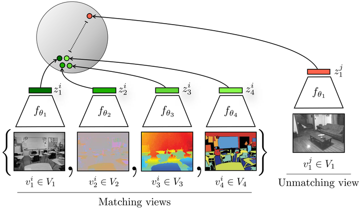
This work was proposed by Yonglong Tian et al. It was built upon the idea of self-supervised contrastive learning frameworks, while CMC adopts multiple views as data (pairs) for contrastive learning pretext.

Contrastive Loss

The contrastive loss between two views $V_1$ (anchor view), $V_2$ is calculated as

$$\mathcal{L}_{contrast}^{V_1,V_2} = - \mathop{\mathbb{E}}_{{v_1^1, v_2^1, \ldots, v_2^{k+1}}}\left[ \log \frac{h_{\theta}({v_1^1, v_2^1})}{\sum_{j=1}^{k+1}h_{\theta}({v_1^1, v_2^j})} \right]$$

and comparing this loss with the k-pair loss, we use $h_\theta$ as similarity function, which is defined as

$$h_{\theta}({v_1,v_2}) = \exp(\frac{f_{\theta_1}(v_1)\cdot f_{\theta_2}(v_2)} {\left\Vert f_{\theta_1}(v_1)\right\Vert \cdot \left\Vert f_{\theta_2}(v_2)\right\Vert} \cdot \frac{1}{\tau})$$

With all the aforementioned information the total contrastive loss between two views is

$$\mathcal{L}\left(V_{1}, V_{2}\right)=\mathcal{L}{\text {contrast}}^{V{1}, V_{2}}+\mathcal{L}{\text {contrast}}^{V{2}, V_{1}}$$

Relation to Information Theory

Here we refer to the concept of Mutual Information, Entropy, Conditional Entropy in Information Theory. A good Information Theory illustration could be found here ⁴.

• An Intuitive Example

  Imagine you met a dog wearing a mask like this.

  You could tell that this is a dog, not a mask, because you not only saw the scene, but also heard its barking, and if you were lucky, you could even tell it’s a dog by feeling its fur.

  So in the example, we use the mutual information in our three senses:

  • visual
  • acoustic
  • touching

  to tell that it’s a dog, so can we exploit the same fashion in the perception of machine as well?

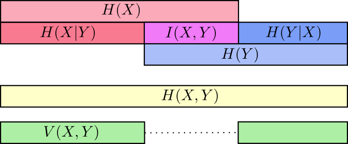
• Mutual Information

  Mutual Information is calculated as $$I(X;Y) = H(X)-H(X|Y)$$

  and applying the formula for entropy and conditional entropy $$\mathrm{I}(X ; Y)=\int_{\mathcal{Y}} \int_{\mathcal{X}} p_{(X, Y)}(x, y) \log \left(\frac{p_{(X, Y)}(x, y)}{p_{X}(x) p_{Y}(y)}\right) d x d y$$

With all these knowledge in mind, the author of CMC contends that the relationship between $\mathcal{L}_{contrast}$ and MI of the representations is

$$\begin{aligned} \mathcal{L}_{\text {contrast }} & \geq \log (k)-\operatorname{E}_{\left(z_{1}, z_{2}\right) \sim p_{z_{1}, z_{2}}(\cdot)} \log \left[\frac{p\left(z_{1}, z_{2}\right)}{p\left(z_{1}\right) p\left(z_{2}\right)}\right] \\ &=\log (k)-I\left(z_{1} ; z_{2}\right) \end{aligned}$$

Moving Mutual Information to the left and contrastive loss to the right we get

$$I\left(v_{i} ; v_{j}\right) \geq I\left(z_{i} ; z_{j}\right) \geq \log (k)-\mathcal{L}_{\text {contrast}}$$

There’s an extra MI term for two views which serves as an upper bound since there are information loss during encoding, i.e. the process $z = f_\theta(v)$.

Therefore, the takeaway message from this part is as follows:

More Mutual Information will be “squeezed out” from two view data $v_1, v_2$ by increasing the number of negatives ($k$) or eliminating the contrastive loss.

In the view of Representation Learning

The aim of CMC is to learn a decent representation of the objects by contrasting multiple views of the objects to the views of other objects. The essence of CMC improving the representation of the objects is that by using CMC, the important information of the object (the mutual information between views for the same object) is embedded in the representation.

So naturally, a question arises, “How many mutual information do we need?” The author explained in a different paper⁵, and the main idea is that, there’s a sweet spot for how many bits of information a specific down-stream task $y$ needs, noted as $I(x;y)$

By training Self-Supervised Contrastive Learning, Mutual Information between views $v_1, v_2$ $I(v_1;v_2)$ is squeezed out, however, once the amount of mutual information (exploited to learn the representation) exceeds the sweet spot for downstream task $y$, the performance will begin to decline.

References