Plot phase portrait with MATLAB and Simulink

Nonlinear Systems

If a system includes one or more nonlinear devices, the system is called a nonlinear system. Every control system is essentially nonlinear. The characteristics of the nonlinear systems can not be described using linear differential equations.

Characteristics of nonlinear systems

• The stablity of a nonlinear system depends on its initial conditions, the inputs to the system, and the system parameters

• There may exist multiple equilibrium in a nonlinear system, in other words, there may have multiple solutions for $\dot{x} = 0$

• The systems may be caught in the state of self-excited oscillation (limit cycle) compared with linear systems

• The outputs of the nonlinear system usually contain additional frequency components and my not contain the original input frequencies.

Analysis and Design Methods of Nonlinear Systems

1. Phase plane (which will be discussed in this article)
2. Describing function
3. MATLAB (implemented in this article)

---

Phase plane anaylsis¹

Phase Plane Analysis is a graphical method for studying first and second-order systems by

• providing motion trajectories corresponding to various initial conditions.

• then examine the qualitative features of the trajectories.

• finally obtaining information regarding the stability and other motion patterns of the system.

---

Example 1

Q: Let’s start with a linear system:

$$\ddot{x} + x = 0$$

Method 1: Calculate by hands with phase plane analysis

First, find the eigenvalues of the characteristic equation: $$ \begin{aligned} &\lambda^{2}+1=0\\ &s_{1,2}=\pm i \end{aligned} $$

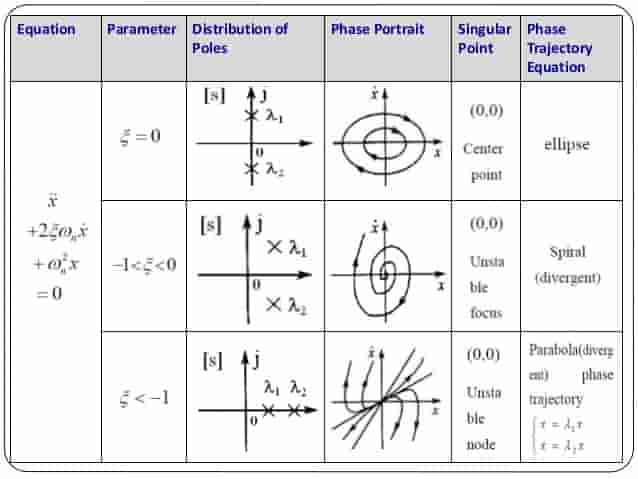
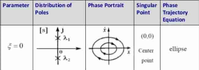
And we know that with such pole distribution, the phase portrait should look like:

Let’s see what we’ll get using MATLAB Simulink

Method 2: Running Simulink simulation

Steps to follow:

1. Find out the input and output
2. Describe the system with basic components, i.e. integrators, gain, etc.
3. Implement the system

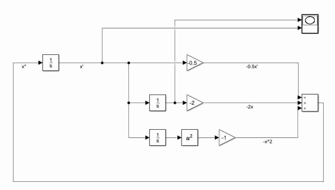
System Topology

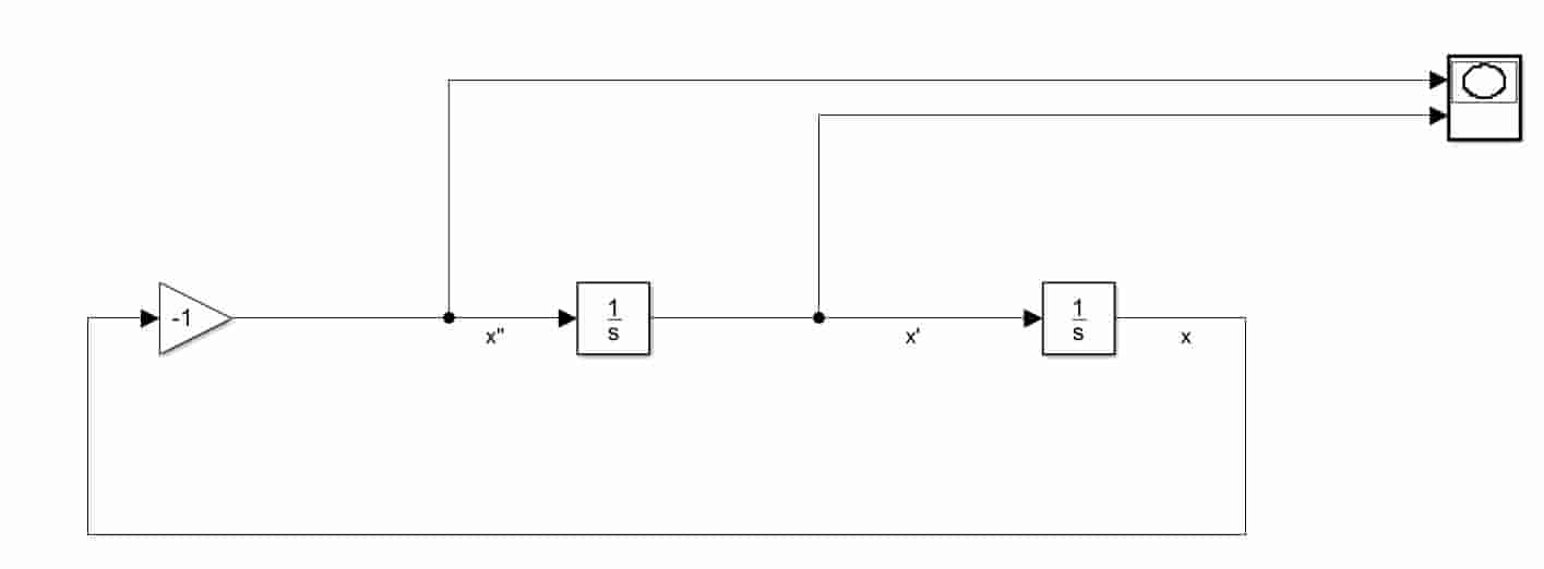
In a second order system, we could cascade integrators in order to get $x, \dot{x}$ and $\ddot{x}$

Since the differential equation of the system is in the form of:

$$\ddot{x} + x = 0$$

we could find out the relationship between $\ddot{x}$ and $x$ by moving $x$ to the right of the equation.

$$\ddot{x} = -x$$

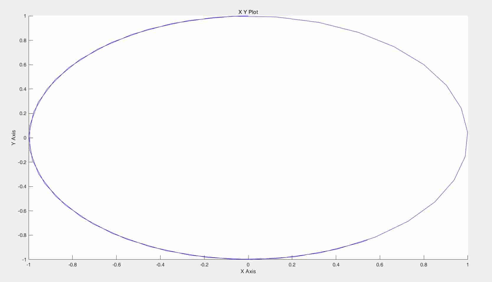
Phase portrait

Example 2

Q: Find the phase portrait of this second-order nonlinear system with such differential equation:

$$ \ddot{x}+0.5 \dot{x}+2 x+x^{2}=0 $$

Leaving $\ddot{x}$ on the left side of the equation, we can get the following equation $$ \ddot{x} = -f(x, \dot{x}) = -0.5\dot{x}-2x-x^2 $$

Method 1: Calculate by hands with phase plane analysis

First, find the singularity points of the system, make

$$ \frac{d \dot{x}}{d x}=-\frac{0.5 \dot{x}+2 x+x^{2}}{\dot{x}}=\frac{0}{0} $$

then we could find our two singularity points

$$ \left\{\begin{array}{l} x=-2 \\ \dot{x}=0 \end{array}\right. $$ and $$ \left\{\begin{array}{l} x=0 \\ \dot{x}=0 \end{array}\right. $$

Therefore, the singularity points of the system lie at $(0, 0)$ and $(-2, 0)$ on the phase plane.

Next, let’s linearize the differential equation $f(\dot{x}, x)$ and then solve for the roots for the equation (also serve as system poles) in order to get the phase portrait.

$$ \left.\frac{\partial f(\dot{x}, x)}{\partial x}\right|_{x=0 \atop \dot{x}=0}=2 x+2=2 $$

$$ \left.\frac{\partial f(\dot{x}, x)}{\partial \dot{x}}\right|_{x=0 \atop \dot{x}=0}=0.5 $$

The linearized system differential equation should look like:

$$ f(\dot{x}, x)=\ddot{x}+0.5 \dot{x}+2x = 0 $$

And the poles are:

$$ s_{1,2}=-0.25\pm 1.39i$$

which means $(0,0)$ is a stable focus.

By the same token, we could get the poles for the other singularity point $(-2, 0)$

$$ s_{1}=1.19$$ $$s_2 = 0.968i$$

Thus, $(-2, 0)$ is a saddle point.

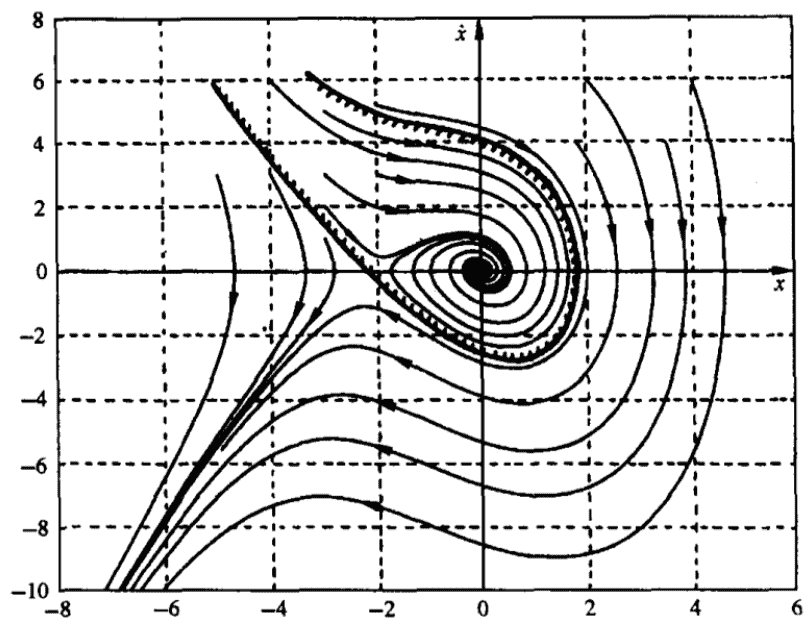
And we know that with such pole distribution, the phase portrait should look like:

Method 2: Running Simulink simulation

Method 3: MATLAB script²

• Step1. First create the file vectfieldn.m in your working directory

  % vectfieldn.m
  % vectfieldn  vector field for system of 2 first order ODEs,
  %            with arrows normalized to the same length
  %   vectfield(func,y1val,y2val) plots the vector field for the system of 
  %   two first order ODEs given by func, using the grid of y1val and 
  %   y2 values given by the vectors y1val and y2val. func is either a 
  %   the name of an inline function of two variables, or a string 
  %   with the name of an m-file.
  %   By default, t=0 is used in func. A t value can be specified as an
  %   additional argument: vectfield(func,y1val,y2val,t)
  function vectfield(func,y1val,y2val,t)
  if nargin==3
    t=0;
  end
  n1=length(y1val);
  n2=length(y2val);
  yp1=zeros(n2,n1);
  yp2=zeros(n2,n1);
  for i=1:n1
    for j=1:n2
      ypv = feval(func,t,[y1val(i);y2val(j)]);
      yp1(j,i) = ypv(1);
      yp2(j,i) = ypv(2);
    end
  end
  len=sqrt(yp1.^2+yp2.^2);
  quiver(y1val,y2val,yp1./len,yp2./len,.6,'r');
  axis tight;
  

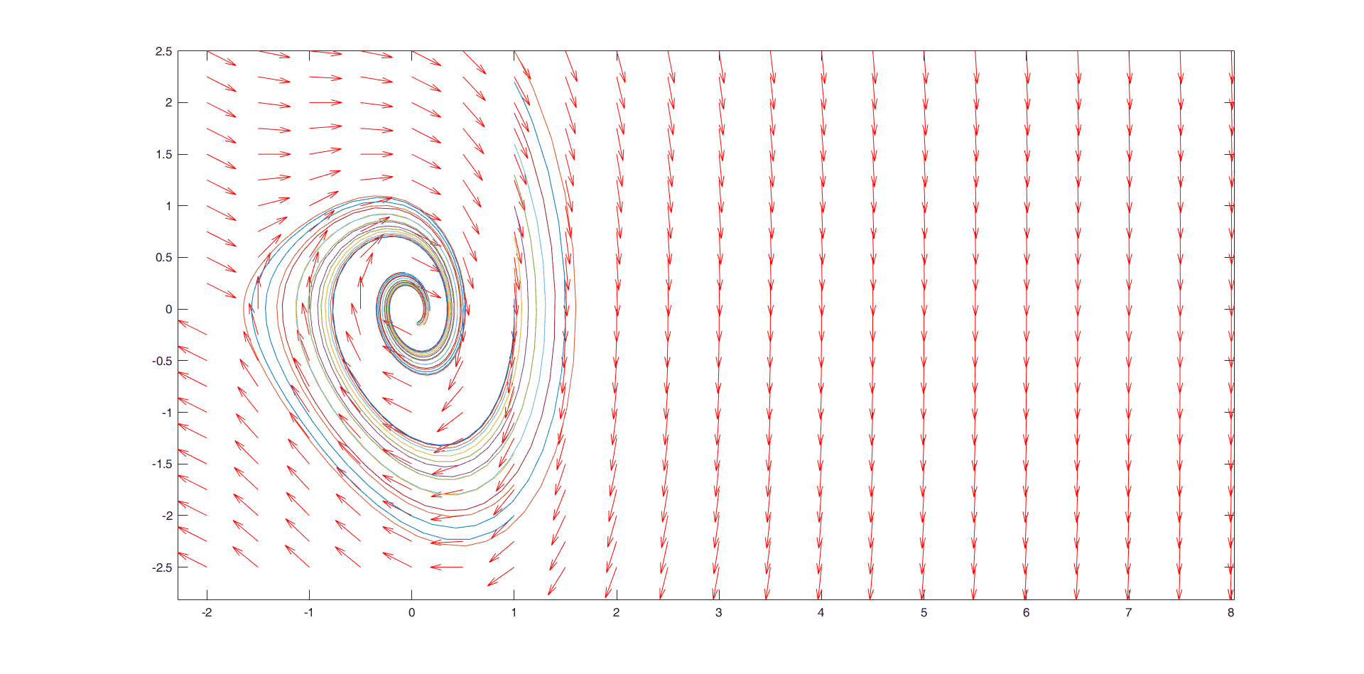
• Step 2. Create another file named main.m and fill in the following code

  % main.m
  % init at (1, y20) where y20 are -2:0.3:2.7 could try other initial points
  f = @(t,y) [y(2);-0.5*y(2)-2*y(1)-y(1)^2]
  vectfieldn(f,-2:.5:8,-2.5:.25:2.5)
  hold on
  for y20=-2:0.3:2.7
    [ts,ys] = ode45(f,[0,10],[1;y20]);
    plot(ys(:,1),ys(:,2))
  end
  hold off